Dimensionality reduction, or dimension reduction, is the transformation of data from a high-dimensional space into a low-dimensional space so that the low-dimensional representation retains some meaningful properties of the original data, ideally close to its intrinsic dimension. Working in high-dimensional spaces can be undesirable for many reasons; raw data are often sparse as a consequence of the curse of dimensionality, and analyzing the data is usually computationally intractable (hard to control or deal with). Dimensionality reduction is common in fields that deal with large numbers of observations and/or large numbers of variables, such as signal processing, speech recognition, neuroinformatics, and bioinformatics.^[1]

Methods are commonly divided into linear and nonlinear approaches.^[1] Approaches can also be divided into feature selection and feature extraction.^[2] Dimensionality reduction can be used for noise reduction, data visualization, cluster analysis, or as an intermediate step to facilitate other analyses.

Feature selection

Feature selection approaches try to find a subset of the input variables (also called features or attributes). The three strategies are: the filter strategy (e.g. information gain), the wrapper strategy (e.g. search guided by accuracy), and the embedded strategy (selected features are added or removed while building the model based on prediction errors).

Data analysis such as regression or classification can be done in the reduced space more accurately than in the original space.^[3]

Feature projection

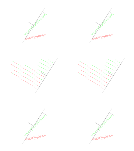
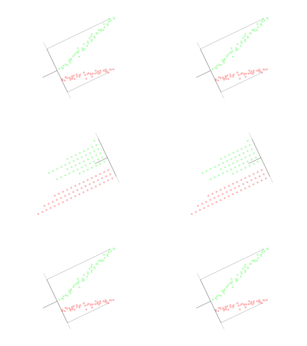
Feature projection (also called feature extraction) transforms the data from the high-dimensional space to a space of fewer dimensions. The data transformation may be linear, as in principal component analysis (PCA), but many nonlinear dimensionality reduction techniques also exist.^[4][5] For multidimensional data, tensor representation can be used in dimensionality reduction through multilinear subspace learning.^[6]

Principal component analysis (PCA)

The main linear technique for dimensionality reduction, principal component analysis, performs a linear mapping of the data to a lower-dimensional space in such a way that the variance of the data in the low-dimensional representation is maximized. In practice, the covariance (and sometimes the correlation) matrix of the data is constructed and the eigenvectors on this matrix are computed. The eigenvectors that correspond to the largest eigenvalues (the principal components) can now be used to reconstruct a large fraction of the variance of the original data. Moreover, the first few eigenvectors can often be interpreted in terms of the large-scale physical behavior of the system, because they often contribute the vast majority of the system's energy, especially in low-dimensional systems. Still, this must be proven on a case-by-case basis as not all systems exhibit this behavior. The original space (with dimension of the number of points) has been reduced (with data loss, but hopefully retaining the most important variance) to the space spanned by a few eigenvectors.^{[citation needed]}

Non-negative matrix factorization (NMF)

NMF decomposes a non-negative matrix to the product of two non-negative ones, which has been a promising tool in fields where only non-negative signals exist,^[7][8] such as astronomy.^[9][10] NMF is well known since the multiplicative update rule by Lee & Seung,^[7] which has been continuously developed: the inclusion of uncertainties,^[9] the consideration of missing data and parallel computation,^[11] sequential construction^[11] which leads to the stability and linearity of NMF,^[10] as well as other updates including handling missing data in digital image processing.^[12]

With a stable component basis during construction, and a linear modeling process, sequential NMF^[11] is able to preserve the flux in direct imaging of circumstellar structures in astronomy,^[10] as one of the methods of detecting exoplanets, especially for the direct imaging of circumstellar discs. In comparison with PCA, NMF does not remove the mean of the matrices, which leads to physical non-negative fluxes; therefore NMF is able to preserve more information than PCA as demonstrated by Ren et al.^[10]

Kernel PCA

Principal component analysis can be employed in a nonlinear way by means of the kernel trick. The resulting technique is capable of constructing nonlinear mappings that maximize the variance in the data. The resulting technique is called kernel PCA.

Graph-based kernel PCA

Other prominent nonlinear techniques include manifold learning techniques such as Isomap, locally linear embedding (LLE),^[13] Hessian LLE, Laplacian eigenmaps, and methods based on tangent space analysis.^[14] These techniques construct a low-dimensional data representation using a cost function that retains local properties of the data, and can be viewed as defining a graph-based kernel for Kernel PCA.

More recently, techniques have been proposed that, instead of defining a fixed kernel, try to learn the kernel using semidefinite programming. The most prominent example of such a technique is maximum variance unfolding (MVU). The central idea of MVU is to exactly preserve all pairwise distances between nearest neighbors (in the inner product space), while maximizing the distances between points that are not nearest neighbors.

An alternative approach to neighborhood preservation is through the minimization of a cost function that measures differences between distances in the input and output spaces. Important examples of such techniques include: classical multidimensional scaling, which is identical to PCA; Isomap, which uses geodesic distances in the data space; diffusion maps, which use diffusion distances in the data space; t-distributed stochastic neighbor embedding (t-SNE), which minimizes the divergence between distributions over pairs of points; and curvilinear component analysis.

A different approach to nonlinear dimensionality reduction is through the use of autoencoders, a special kind of feedforward neural networks with a bottle-neck hidden layer.^[15] The training of deep encoders is typically performed using a greedy layer-wise pre-training (e.g., using a stack of restricted Boltzmann machines) that is followed by a finetuning stage based on backpropagation.

Linear discriminant analysis (LDA)

Linear discriminant analysis (LDA) is a generalization of Fisher's linear discriminant, a method used in statistics, pattern recognition and machine learning to find a linear combination of features that characterizes or separates two or more classes of objects or events.

Generalized discriminant analysis (GDA)

GDA deals with nonlinear discriminant analysis using kernel function operator. The underlying theory is close to the support-vector machines (SVM) insofar as the GDA method provides a mapping of the input vectors into high-dimensional feature space.^[16][17] Similar to LDA, the objective of GDA is to find a projection for the features into a lower dimensional space by maximizing the ratio of between-class scatter to within-class scatter.

Autoencoder

Autoencoders can be used to learn nonlinear dimension reduction functions and codings together with an inverse function from the coding to the original representation.

t-SNE

T-distributed Stochastic Neighbor Embedding (t-SNE) is a nonlinear dimensionality reduction technique useful for visualization of high-dimensional datasets. It is not recommended for use in analysis such as clustering or outlier detection since it does not necessarily preserve densities or distances well.^[18]

UMAP

Uniform manifold approximation and projection (UMAP) is a nonlinear dimensionality reduction technique. Visually, it is similar to t-SNE, but it assumes that the data is uniformly distributed on a locally connected Riemannian manifold and that the Riemannian metric is locally constant or approximately locally constant.

Dimension reduction

For high-dimensional datasets (i.e. with number of dimensions more than 10), dimension reduction is usually performed prior to applying a K-nearest neighbors algorithm (k-NN) in order to avoid the effects of the curse of dimensionality.^[19]

Feature extraction and dimension reduction can be combined in one step using principal component analysis (PCA), linear discriminant analysis (LDA), canonical correlation analysis (CCA), or non-negative matrix factorization (NMF) techniques as a pre-processing step followed by clustering by K-NN on feature vectors in reduced-dimension space. In machine learning this process is also called low-dimensional embedding.^[20]

For very-high-dimensional datasets (e.g. when performing similarity search on live video streams, DNA data or high-dimensional time series) running a fast approximate K-NN search using locality-sensitive hashing, random projection,^[21] "sketches",^[22] or other high-dimensional similarity search techniques from the VLDB conference toolbox might be the only feasible option.

Applications

A dimensionality reduction technique that is sometimes used in neuroscience is maximally informative dimensions,^{[citation needed]} which finds a lower-dimensional representation of a dataset such that as much information as possible about the original data is preserved.